GeneticsMakie.jl

versioninfo()

Julia Version 1.7.0
Commit 3bf9d17731 (2021-11-30 12:12 UTC)
Platform Info:
  OS: macOS (x86_64-apple-darwin19.5.0)
  CPU: Intel(R) Core(TM) i9-9880H CPU @ 2.30GHz
  WORD_SIZE: 64
  LIBM: libopenlibm
  LLVM: libLLVM-12.0.1 (ORCJIT, skylake)

Why Makie.jl?

1. Plotting millions of data points is easy

LD structure for ~66,000 SNPs in the MHC region → ≈2 billion unique data points

For more information on the MHC, see Horton et al. 2004

2. Plotting figures with complex layouts is easy

Publication-quality figure generated using Makie.jl's default layout tools w/o further modifications (e.g. in Illustrator)

Looks interesting? Check out Makie.jl documentation!

Why GeneticsMakie.jl?

• The purpose of GeneticsMakie.jl is to facilitate visualization and interpretation of genetic association results
• This is achieved by visualizing $\geq 100$s of genetic and genomic data simultaneously
• GeneticsMakie.jl is supposed to work with other OpenMendel (e.g. SnpArrays.jl) and Julia Data Science (e.g. DataFrames.jl) packages

Example phenome-scale LocusZoom plots

GRIN2A is a high-confidence schizophrenia risk gene

MHC region is one of the most pleiotropic regions in the human genome

Looks intriguing? Check out GeneticsMakie.jl documentation!

Example code for ADAMTSL3 locus in inguinal hernia

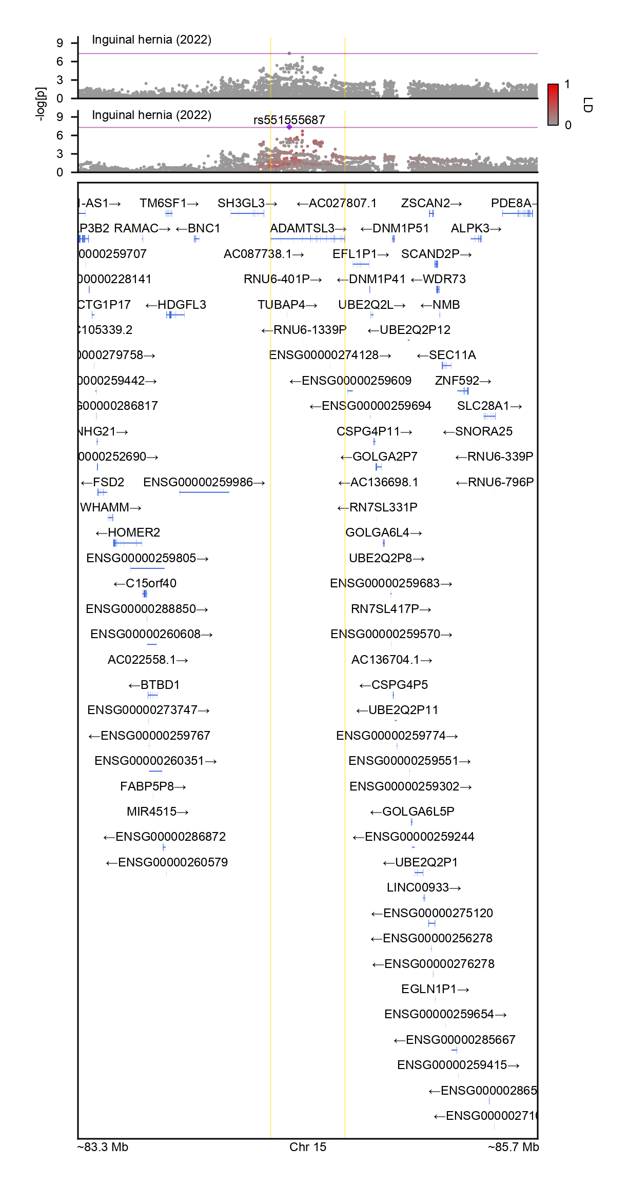
Visualizing the backbone of a LocusZoom plot requires genetic association data, gene annotation data, and LD reference panel

• GWAS summary statistics can be downloaded from Danish National Biobank portal
• For gene annotation, we can use GENCODE v39
• For LD reference panel, we can use 1000 Genomes Project

using GeneticsMakie, CairoMakie, CSV, DataFrames, SnpArrays

set_theme!(font = "Arial")

@info "Loading GENCODE v39 annotation for chromosome 15"
@time gencode = CSV.read("./gencode.v39lift37.annotation.chr15.gtf.gz", DataFrame,
    header = ["seqnames", "source", "feature", "start", "end", "score", "strand", "phase", "info"],
    delim = "\t", skipto = 6)
gencode[!, :info]

  6.724185 seconds (3.57 M allocations: 269.634 MiB, 1.38% gc time, 94.54% compilation time)

┌ Info: Loading GENCODE v39 annotation for chromosome 15
└ @ Main In[4]:1

117418-element Vector{String}:
 "gene_id \"ENSG00000215567.5_1\"; " ⋯ 454 bytes ⋯ "\"; remap_status \"full_contig\";"
 "gene_id \"ENSG00000215567.5_1\"; " ⋯ 454 bytes ⋯ "\"; remap_status \"full_contig\";"
 "gene_id \"ENSG00000215567.5_1\"; " ⋯ 454 bytes ⋯ "\"; remap_status \"full_contig\";"
 "gene_id \"ENSG00000201241.1\"; ge" ⋯ 122 bytes ⋯ "stituted_missing_target \"V38\";"
 "gene_id \"ENSG00000201241.1\"; tr" ⋯ 255 bytes ⋯ "stituted_missing_target \"V38\";"
 "gene_id \"ENSG00000201241.1\"; tr" ⋯ 299 bytes ⋯ "stituted_missing_target \"V38\";"
 "gene_id \"ENSG00000258463.1_1\"; " ⋯ 160 bytes ⋯ "remap_target_status \"overlap\";"
 "gene_id \"ENSG00000258463.1_1\"; " ⋯ 404 bytes ⋯ "remap_target_status \"overlap\";"
 "gene_id \"ENSG00000258463.1_1\"; " ⋯ 450 bytes ⋯ "\"; remap_status \"full_contig\";"
 "gene_id \"ENSG00000274347.1_1\"; " ⋯ 158 bytes ⋯ " 1; remap_target_status \"new\";"
 "gene_id \"ENSG00000274347.1_1\"; " ⋯ 404 bytes ⋯ "g\"; remap_target_status \"new\";"
 "gene_id \"ENSG00000274347.1_1\"; " ⋯ 454 bytes ⋯ "\"; remap_status \"full_contig\";"
 "gene_id \"ENSG00000188403.7_1\"; " ⋯ 166 bytes ⋯ "remap_target_status \"overlap\";"
 ⋮
 "gene_id \"ENSG00000248472.8_1\"; " ⋯ 429 bytes ⋯ "\"; remap_status \"full_contig\";"
 "gene_id \"ENSG00000248472.8_1\"; " ⋯ 429 bytes ⋯ "\"; remap_status \"full_contig\";"
 "gene_id \"ENSG00000248472.8_1\"; " ⋯ 381 bytes ⋯ "remap_target_status \"overlap\";"
 "gene_id \"ENSG00000248472.8_1\"; " ⋯ 429 bytes ⋯ "\"; remap_status \"full_contig\";"
 "gene_id \"ENSG00000248472.8_1\"; " ⋯ 429 bytes ⋯ "\"; remap_status \"full_contig\";"
 "gene_id \"ENSG00000248472.8_1\"; " ⋯ 429 bytes ⋯ "\"; remap_status \"full_contig\";"
 "gene_id \"ENSG00000248472.8_1\"; " ⋯ 461 bytes ⋯ "remap_target_status \"overlap\";"
 "gene_id \"ENSG00000248472.8_1\"; " ⋯ 509 bytes ⋯ "\"; remap_status \"full_contig\";"
 "gene_id \"ENSG00000248472.8_1\"; " ⋯ 509 bytes ⋯ "\"; remap_status \"full_contig\";"
 "gene_id \"ENSG00000248472.8_1\"; " ⋯ 509 bytes ⋯ "\"; remap_status \"full_contig\";"
 "gene_id \"ENSG00000248472.8_1\"; " ⋯ 509 bytes ⋯ "\"; remap_status \"full_contig\";"
 "gene_id \"ENSG00000248472.8_1\"; " ⋯ 509 bytes ⋯ "\"; remap_status \"full_contig\";"

The :info column in GENCODE gtf file contains rich information about each gene/isoform

GeneticsMakie.parsegtf!(gencode)
names(gencode)

14-element Vector{String}:
 "seqnames"
 "source"
 "feature"
 "start"
 "end"
 "score"
 "strand"
 "phase"
 "info"
 "gene_id"
 "gene_name"
 "gene_type"
 "transcript_id"
 "transcript_support_level"

select!(gencode, :seqnames, :feature, :start, :end, :strand, :gene_id, :gene_name, :gene_type, :transcript_id)
@assert size(gencode) == (117_418, 9)

@info "Loading 1000 Genomes European reference panel for chromosome 15"
kgp = SnpData("./kgp.chr15")
@assert size(kgp) == (503, 200_311)

┌ Info: Loading 1000 Genomes European reference panel for chromosome 15
└ @ Main In[7]:1

@info "Loading GWAS results for chromosome 15"
gwas = CSV.read("./hernia.chr15.gz", DataFrame, comment = "##", missingstring = "NA")

┌ Info: Loading GWAS results for chromosome 15
└ @ Main In[8]:1

299,624 rows × 8 columns

	CHR	POS	SNPID	Allele1	Allele2	AFAllele2	BETA	p
	Int64	Int64	String	String	String	Float64	Float64	Float64
1	15	20001226	rs28896870	C	T	0.113114	0.0110027	0.487073
2	15	20001774	rs28812614	T	C	0.257554	0.0216504	0.0621705
3	15	20004721	rs145629091	A	G	0.137294	0.0259993	0.0793635
4	15	20014120	rs12594432	G	A	0.138131	0.0267138	0.0689262
5	15	20017513	rs12900040	T	C	0.118101	0.0100042	0.522537
6	15	20021591	rs11535026	T	A	0.116481	0.00981448	0.531855
7	15	20021749	rs12595413	C	T	0.137905	0.0264183	0.0724226
8	15	20026191	rs533345786	A	AAAG	0.111671	0.0109291	0.504701
9	15	20026200	rs543944619	A	C	0.112151	0.010696	0.511987
10	15	20026202	rs565344963	G	A	0.112151	0.010696	0.511987
11	15	20026205	rs533002721	A	T	0.112476	0.0107821	0.507315
12	15	20026208	rs12900467	T	C	0.112476	0.0107821	0.507315
13	15	20027647	rs8029999	C	G	0.122335	0.00816835	0.817027
14	15	20028363	rs74485484	A	G	0.117248	0.0102801	0.50935
15	15	20028762	rs12903976	C	T	0.114862	0.00984186	0.535829
16	15	20029688	rs34390178	C	G	0.134265	0.0296249	0.0493136
17	15	20030951	rs35979813	T	C	0.116333	0.0104721	0.489063
18	15	20031739	rs12442841	T	G	0.115869	0.0106059	0.485068
19	15	20034803	rs144043507	C	T	0.13777	0.0270265	0.0665972
20	15	20034919	rs78737532	T	C	0.115742	0.010556	0.487632
21	15	20039239	rs12439778	A	G	0.116222	0.0099177	0.509795
22	15	20039935	rs71464559	T	A	0.258699	0.0223527	0.0491104
23	15	20040322	rs199772085	A	G	0.10038	0.0129446	0.442101
24	15	20040573	rs12439263	T	A	0.117796	0.0093258	0.534502
25	15	20040668	rs193121394	G	A	0.138654	0.0268971	0.065546
26	15	20042094	rs12592301	C	T	0.256431	0.0219884	0.0644688
27	15	20044198	rs28535042	T	C	0.259195	0.0222399	0.0619445
28	15	20044342	rs117764863	G	A	0.0568624	0.00119022	0.955402
29	15	20044383	rs35261146	C	T	0.116351	0.00980477	0.511018
30	15	20045025	rs36028981	G	A	0.116646	0.00983351	0.510217
⋮	⋮	⋮	⋮	⋮	⋮	⋮	⋮	⋮

GeneticsMakie.mungesumstats!(gwas)

loci = GeneticsMakie.findgwasloci(gwas)

1 rows × 3 columns

	CHR	BP	P
	String	Int64	Float64
1	15	84419314	4.24936e-8

GCTA-COJO is planned to be implemented in the future for findgwasloci

GeneticsMakie.findgwasloci(gwas; p = 1e-6)

2 rows × 3 columns

	CHR	BP	P
	String	Int64	Float64
1	15	84419314	4.24936e-8
2	15	67467297	2.48762e-7

GeneticsMakie.findclosestgene(loci, gencode)

1 rows × 4 columns

	CHR	BP	gene	distance
	String	Int64	String	Int64
1	15	84419314	TUBAP4	10363

GeneticsMakie.findclosestgene(loci, gencode; start = true)

1 rows × 4 columns

	CHR	BP	gene	distance
	String	Int64	String	Int64
1	15	84419314	TUBAP4	10778

GeneticsMakie.findclosestgene(loci, gencode; proteincoding = true)

1 rows × 4 columns

	CHR	BP	gene	distance
	String	Int64	String	Int64
1	15	84419314	ADAMTSL3	96474

loci = GeneticsMakie.findclosestgene(loci, gencode; start = true, proteincoding = true)

1 rows × 4 columns

	CHR	BP	gene	distance
	String	Int64	String	Int64
1	15	84419314	ADAMTSL3	96474

function locuszoom(genes)
    for gene in genes
        @info "Working on $gene gene"
        window = 1e6
        chr, start, stop = GeneticsMakie.findgene(gene, gencode)
        range1, range2 = start - window, stop + window
        gwas_subset = gwas[findall((gwas.CHR .== chr) .& (gwas.BP .>= range1) .& (gwas.BP .<= range2)), :]
        @info "Plotting LocusZoom"
        f = Figure(resolution = (306, 792))
        axs = [Axis(f[i, 1]) for i in 1:3]
        GeneticsMakie.plotlocus!(axs[1], chr, range1, range2, gwas_subset)
        GeneticsMakie.plotlocus!(axs[2], chr, range1, range2, gwas_subset; ld = kgp)
        for i in 1:2
            Label(f[i, 1, Top()], "Inguinal hernia (2022)", textsize = 6, halign = :left, padding = (7.5, 0, -5, 0))
            rowsize!(f.layout, i, 30)
        end
        rs = GeneticsMakie.plotgenes!(axs[3], chr, range1, range2, gencode; height = 0.1)
        rowsize!(f.layout, 3, rs)
        GeneticsMakie.labelgenome(f[3, 1, Bottom()], chr, range1, range2)
        Colorbar(f[1:2, 2], limits = (0, 1), ticks = 0:1:1, height = 20,
            colormap = (:gray60, :red2), label = "LD", ticksize = 0, tickwidth = 0,
            tickalign = 0, ticklabelsize = 6, flip_vertical_label = true,
            labelsize = 6, width = 5, spinewidth = 0.5)
        Label(f[1:2, 0], text = "-log[p]", textsize = 6, rotation = pi / 2)
        for i in 1:3
            vlines!(axs[i], start, color = (:gold, 0.5), linewidth = 0.5)
            vlines!(axs[i], stop, color = (:gold, 0.5), linewidth = 0.5)
        end
        for i in 1:2
            lines!(axs[i], [range1, range2], fill(-log(10, 5e-8), 2), color = (:purple, 0.5), linewidth = 0.5)
        end
        rowgap!(f.layout, 5)
        colgap!(f.layout, 5)
        resize_to_layout!(f)
        save("./$(gene)-locuszoom.png", f, px_per_unit = 4)
    end
end

@time locuszoom(loci.gene)

 73.092486 seconds (245.55 M allocations: 12.107 GiB, 3.10% gc time, 83.83% compilation time)

┌ Info: Working on ADAMTSL3 gene
└ @ Main In[16]:3
┌ Info: Plotting LocusZoom
└ @ Main In[16]:8

@time locuszoom(loci.gene)

 10.318701 seconds (57.06 M allocations: 2.102 GiB, 3.77% gc time)

┌ Info: Working on ADAMTSL3 gene
└ @ Main In[16]:3
┌ Info: Plotting LocusZoom
└ @ Main In[16]:8

An example workflow for phenome-scale LocusZoom

Hypothetical scenario: you have run a GWAS and would like to visualize genome-wide significant loci automatically with 100s of GWAS results and functional genomic annotations

1. Munge GWAS summary statistics (using mungesumstats! function)
2. Save each GWAS result as an Arrow or Parquet file (using Arrow.jl or Parquet.jl)
3. Find GWAS loci for your phenotypes of interest (using findgwasloci function)
4. Iterate through GWAS loci, subsetting genomic regions from Arrow or Parquet files (using DataFrames.jl)
5. Add other functional genomic data as separate layers as needed

Checkout example code!

Other functionalities

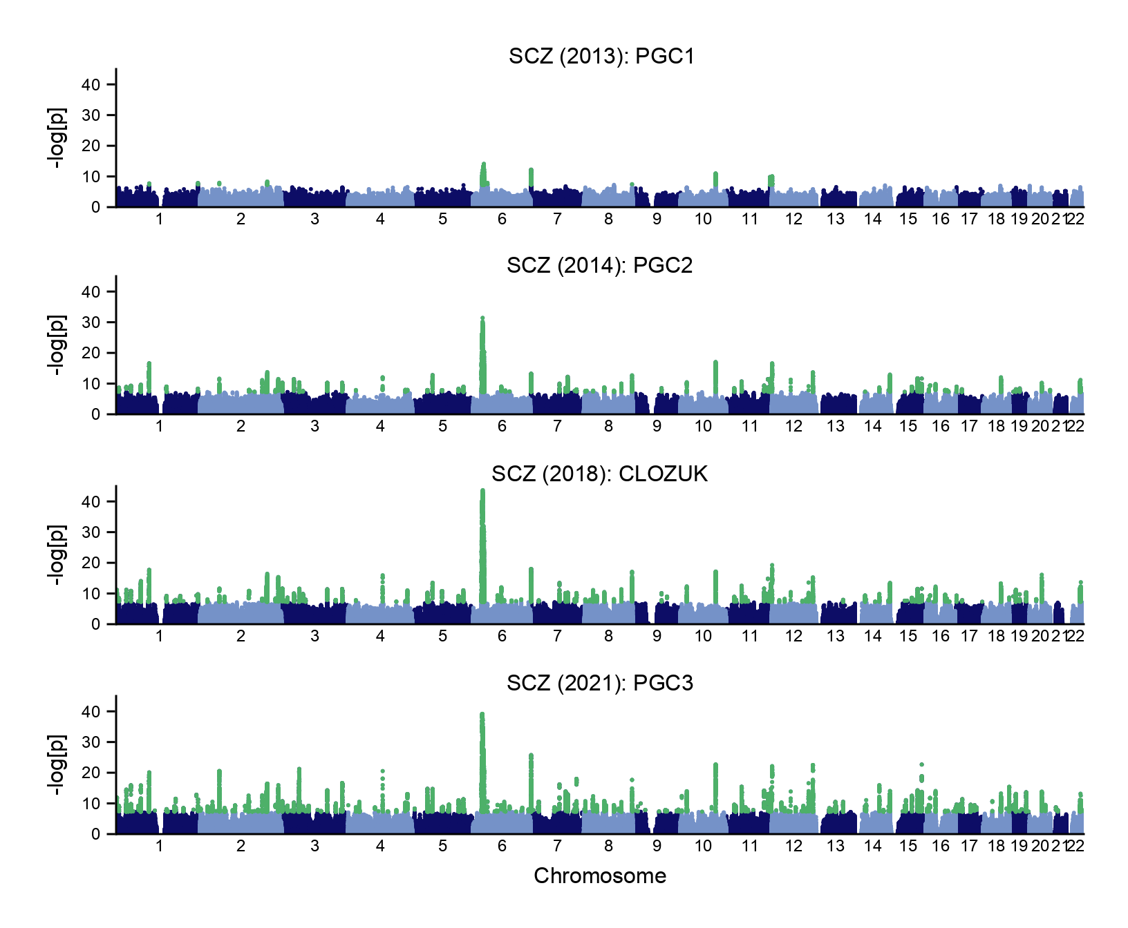
An increase in sample size has led to many more dicovery of GWAS loci for schizophrenia