Julia for Data Science
# for reproducibility
versioninfo()
From previous two tutorials, we practiced a few essential data wrangling steps in R and Python.
Pipes
Data ingestion
Data filtering (rows) and selection (columns)
Data sorting and ranking
Data merging (joins)
Mutate (dplyr) or transform (Julia)
Pivot (dplyr) or reshape (Julia)
Group by
Data summaries
Visualization
The Julia package DataFrames.jl is the analog of dplyr and data.table in R and panda in Python.
Optional reading: Comparison of DataFrames.jl with Python/R/Stata.
using AlgebraOfGraphics, CairoMakie, CSV, DataFrames, Dates, Pipe
# path to MIMIC data
mimic_path = Sys.islinux() ? "/home/shared/1.0" : "/Users/huazhou/Desktop/mimic-iv-1.0"
# for printing all columns of DataFrame
ENV["COLUMNS"] = 1000
Data ingestion
Plain text files can be parsed by the CSV.jl package.
icustays_tbl
We use the dateformat argument to correctly parse charttime as DateTime.
icustays_tbl = CSV.File(
    mimic_path * "/icu/icustays.csv.gz",
    dateformat = "yyyy-mm-dd HH:MM:SS"
    ) |> DataFrame
admissions_tbl
admissions_tbl = CSV.File(
    mimic_path * "/core/admissions.csv.gz",
    dateformat = "yyyy-mm-dd HH:MM:SS"
    ) |> DataFrame
patients_tbl
patients_tbl = CSV.File(mimic_path * "/core/patients.csv.gz") |> DataFrame
chartevents_tbl
We use the dataformat argument to correctly parse charttime as DateTime.
@time chartevents_tbl = CSV.File(
    mimic_path * "/icu/chartevents_filtered_itemid.csv.gz",
    dateformat = "yyyy-mm-dd HH:MM:SS"
    ) |>
    DataFrame
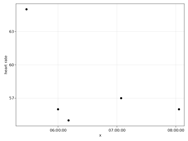
Let's visualize the heart rate readings for a specific stay.
#filter(row -> row.stay_id == 30600691 && row.itemid == 220045, chartevents_tbl) |>
chartevents_subset = @pipe chartevents_tbl |>
    filter(row -> row.stay_id == 30600691 && row.itemid == 220045, _) |>
    select(_, [:charttime, :valuenum]) |>
    DataFrame
# be patient: time-to-first-plot is long!
x = chartevents_subset[!, :charttime]
y = chartevents_subset[!, :valuenum]
df = (; x, y)
plt = data(df) *
    mapping(:x, [:y] .=> "heart rate") *
    visual(Scatter)
draw(plt)
Target cohort (from R session)
Let's continue on with the task we did with R. We aim to develop a predictive model, which computes the chance of dying within 30 days of ICU stay intime based on baseline features
first_careunitageatintimegenderethnicity- first measurement of the following vitals since ICU stay
intime- 220045 for heart rate
- 223761 for Temperature Fahrenheit
We restrict to the first ICU stays of each unique patient.
Wrangling and merging data frames
Our stragegy is
Identify and keep the first ICU stay of each patient.
Identify and keep the first vital measurements during the first ICU stay of each patient.
Join four data frames into a single data frame.
Important data wrangling concepts: group_by, sort, slice, joins, and pivot.
Step 1: restrict to the first ICU stay of each patient
icustays_df has 76,540 rows, which is reduced to 53,150 unique ICU stays.
icustays_tbl_1ststay = @pipe icustays_tbl |>
    sort(_, [:subject_id, :intime]) |>
    unique(_, :subject_id)
Step 2: restrict to the first vital measurements during the ICU stay
Key data wrangling concepts: select, left_join, right_join, group_by, arrange, pivot.
@time chartevents_tbl_1ststay = @pipe chartevents_tbl |>
    # pull in the intime/outtime of each ICU stay
    rightjoin(_, select(icustays_tbl_1ststay, :stay_id, :intime, :outtime), on = :stay_id) |>
    # only keep items during this ICU intime
    filter(row -> ismissing(row.charttime) ? false : (row.charttime ≥ row.intime && row.charttime ≤ row.outtime), _) |>
    # only keep the first charttime for each stay_id x item
    sort(_, [:stay_id, :itemid, :charttime]) |>
    unique(_, [:stay_id, :itemid]) |>
    # do not need charttime, intime and outtime anymore
    select(_, Not([:charttime, :intime, :outtime])) |>
    # pivot_wider (R) or reshape (Julia)
    unstack(_, [:subject_id, :hadm_id, :stay_id], :itemid, :valuenum) |>
    # more informative column names
    rename(_, Dict(
        "220045" => "heart_rate",
        "223761" => "temp_f",
        ))
Step 3: merge data frames
New data wrangling concept: mutate.
@time mimic_icu_cohort = @pipe icustays_tbl_1ststay |>
    # merge data frames
    leftjoin(_, admissions_tbl, on = [:subject_id, :hadm_id]) |>
    leftjoin(_, patients_tbl, on = [:subject_id]) |>
    leftjoin(_, chartevents_tbl_1ststay, on = [:stay_id, :subject_id, :hadm_id]) |>
    # age_intime is the age at ICU stay intime
    insertcols!(_, :age_intime => _.anchor_age .+ year.(_.intime) .- _.anchor_year) |>
    # whether the patient died within 30 days of ICU stay intime
    insertcols!(_, :hadm_to_death => _.deathtime .- _.intime) |>
    insertcols!(_, :thirty_day_mort => _.hadm_to_death .≤ Millisecond(2592000000))
# missing in thirty_day_mort means patient not die
replace!(mimic_icu_cohort.thirty_day_mort, missing => false)
mimic_icu_cohort
Data visualization
It is always a good idea to visualize data as much as possible before any statistical analysis.
Remember we want to model:
thirty_day_mort ~ first_careunit + age_intime + gender + ethnicity + heart_rate + temp_f
Let's start with a numerical summary of variables of interest.
@pipe mimic_icu_cohort |>
    select(_, [
        :first_careunit,
        :gender,
        :ethnicity,
        :age_intime,
        :heart_rate,
        :temp_f,
        :thirty_day_mort
        ]) |>
    describe(_)
Univariate summaries
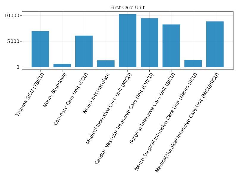
Bar plot of first_careunit.
@pipe mimic_icu_cohort |>
    groupby(_, :first_careunit) |>
    combine(_, nrow) |>
    barplot(
        _.first_careunit.refs,
        _.nrow,
        axis = (xticks = (1:size(_, 1), _.first_careunit), title = "First Care Unit", xticklabelrotation = 45.0)
)
Bivariate summaries
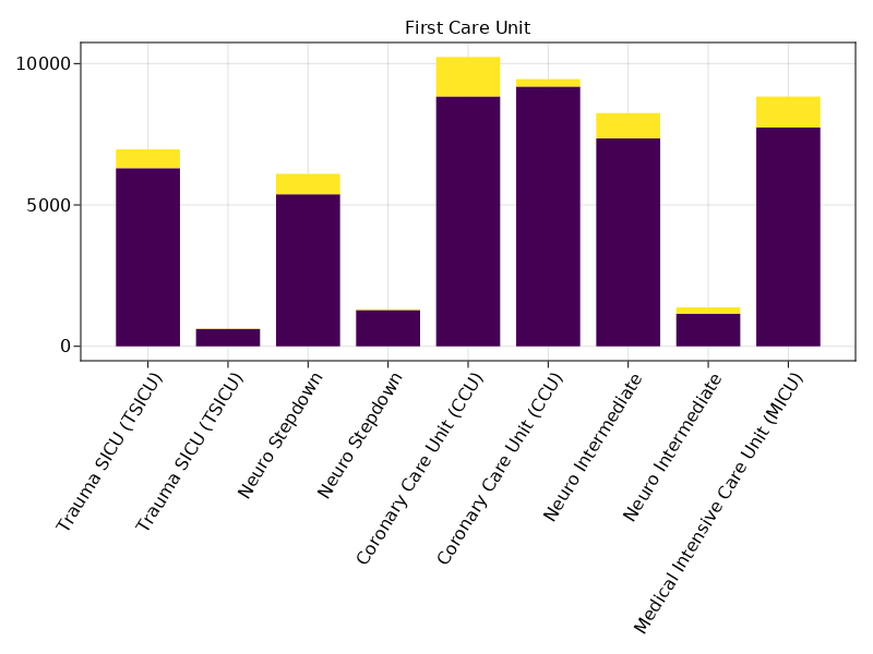
Tally of thirty_day_mort vs first_careunit.
@pipe mimic_icu_cohort |>
    groupby(_, [:first_careunit, :thirty_day_mort]) |>
    combine(_, nrow) |>
    disallowmissing(_, :thirty_day_mort) |>
    barplot(
        _.first_careunit.refs,
        _.nrow,
        stack = _.thirty_day_mort,
        color = _.thirty_day_mort,
        axis = (xticks = (1:size(_, 1), _.first_careunit), title = "First Care Unit", xticklabelrotation = 45.0)
    )
Pros and Cons of Julia
Pros
Julia solves the notorious two language problem in scientific computing. Julia combines the functionality and ease of use of Python, R, Matlab, SAS and Stata with the speed of C/C++ and Java. News: Julia Joins Petaflop Club.
As a new language, Julia integrates well with modern hardware (GPUs, parallel and distributed computing).
Excel domains such as differential equations, auto-differentiation, and optimization.
Interoperability with other languages (Python, R, Matlab, C, C++, Fortran).
Cons
Smaller ecosystem? Not anymore. On the contrary, some ecosystems (e.g., plotting, auto-diff, DL) are too rich/confusing for user to choose.
Smaller user base, compared to Python and R.
Lack of IDEs as feature-rich as RStudio.
Compilation time of some packages (Plots.jl, LoopVectorization.jl, etc) can be long. Time-to-first-plot issue